Feist-Khovratovich technique for computing KZG proofs fast

tl;dr: Given a polynomial $f(X)$ of degree $m$, can we compute all $n$ KZG proofs for $f(\omega^k), k\in[0,n-1]$ in $O(n\log{n})$ time, where $\omega$ is a primitive $n$th root of unity? Dankrad Feist and Dmitry Khovratovich¹ give a resounding ‘yes!’

$$ \def\Adv{\mathcal{A}} \def\Badv{\mathcal{B}} \def\vect#1{\mathbf{#1}} %\definecolor{myBlueColor}{HTML}{268BD2} %\definecolor{myPinkColor}{HTML}{D33682} %\definecolor{myGreenColor}{HTML}{859900} %\def\mygreen#1{\color{myGreenColor}{#1}} %\def\mygreen#1{\color{green}{#1}} %\newcommand{\myblue}[1]{\textcolor{myBlueColor}{#1}} %\newcommand{\mypink}[1]{\textcolor{myPinkColor}{#1}} $$

Preliminaries

First, read:

• Basics of polynomials
• The Discrete Fourier Transform (DFT) for $n$th roots of unity
• KZG polynomial commitments

Notation:

• $g$ generates a “bilinear” group $\Gr$ of prime order $p$, endowed with a bilinear map or pairing $e : \Gr\times\Gr\rightarrow\Gr_T$
  • we use multiplicative notation here: i.e., $g^a$ denotes composing $g$ with itself $a$ times
• there exists a primitive $n$th root of unity $\omega$, where $n$ is a power of two
• we have $q$-SDH public parameters $\left(g, g^\tau,g^{\tau^2},\dots,g^{\tau^q}\right)$, for $q \le n$
• we work with polynomials in $\Zp[X]$ of degree $\le n$

Related work

Other works that give related techniques to compute proofs fast in KZG-like polynomial commitments are:

• Authenticated multipoint evaluation trees (AMTs) (see paper² and blogpost)
• “How to compute all Pointproofs” (see paper³), much inspired by Feist and Khovratovich’s technique explained in this blogpost

Refresher: Computing $n$ different KZG proofs

Let $f(X)$ be a polynomial with coefficients $f_i$:

\begin{align*} f(X) &= f_m X^m + f_{m-1} X^{m-1} + \cdots f_1 X + f_0\\
&= \sum_{i\in[0,m]} f_i X^i \end{align*}

Recall that a KZG evaluation proof $\pi_i$ for $f(\omega^i)$ is a KZG commitment to a quotient polynomial $Q_i(X) = \frac{f(X) - f(\omega^i)}{X-\omega^i}$: \begin{align*} \pi_i = g^{Q_i(\tau)} = g^{\frac{f(\tau) - f(\omega^i)}{\tau-\omega^i}} \end{align*}

Computing such a proof takes $O(m)$ time!

But what if we want to compute all $\pi_i, i\in[0, n)$?

If done naively, this would take $O(nm)$ time, which is too expensive!

Lower bound? Is this $O(nm)$ time complexity inherent? After all, to compute $\pi_i$ don’t we first need to compute $Q_i(X)$, which takes $O(m)$ time? As you’ll see below, the answer is “no!”

Fortunately, Feist and Khovratovich observe that the $Q_i$’s are algebraically-related and so are their $\pi_i$ KZG commitments! As a result, they observe that computing all $\pi_i$’s does not require computing all $Q_i$’s.

Below, we explain how their faster, $O(n\log{n})$-time technique works!

An important caveat is that their technique relies on the evaluation points being $\omega^0,\dots,\omega^{n-1}$.

Quotient polynomials and their coefficients

To understand how the $\pi_i$’s relate to one other, let us look at the coefficients of $Q_i(X)$.

We can show that when dividing $f$ (of degree $m$) by $(X-\omega^i)$ we obtain a quotient polynomial with coefficients $t_0, t_1, \dots, t_{m-1}$ such that: \begin{align} \label{eq:div-coeffs-1} t_{m-1} &= f_m\\
%t_{m-2} &= f_{m-1} + \omega^i \cdot f_m\\
%t_{m-3} &= f_{m-2} + \omega^i \cdot t_{m-2}\\
% &= f_{m-2} + \omega^i \cdot (f_{m-1} + \omega^i \cdot f_m)\\
% &= f_{m-2} + \omega^i \cdot f_{m-1} + \omega^{2i} \cdot f_m\\
%t_{m-4} &= f_{m-3} + \omega^i \cdot t_{m-3}\\
% &= f_{m-3} + \omega^i \cdot (f_{m-2} + \omega^i \cdot f_{m-1} + \omega^{2i} \cdot f_m)\\
% &= f_{m-3} + \omega^i \cdot f_{m-2} + \omega^{2i} \cdot f_{m-1} + \omega^{3i} \cdot f_m\\\ % & \vdots\\
\label{eq:div-coeffs-2} t_{j} &= f_{j+1} + \omega^i \cdot t_{j+1}, \forall j \in [0, m-1) % & \vdots\\
% t_0 &= f_1 + \omega^i \cdot f_2 + \omega^{2i} f_3 + \dots + \omega^{m-1} f_m \end{align} Note that the $t_i$’s are a function of $f_m, f_{m-1},\dots, f_1$, but not of $f_0$!

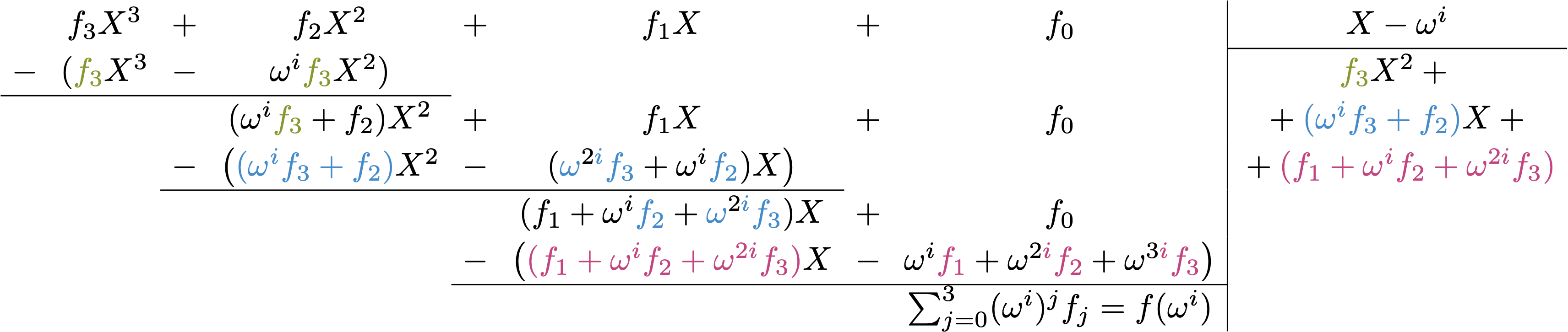
Proof: One could prove by induction that the coefficients above are correct. However, it's easiest to take an example and convince yourself, as shown below for $m=4$. (Click to expand.)

Indeed, the quotient obtained when dividing $f(X) = f_3 X^3 + f_2 X^2 + \dots + f_0$ by $X-\omega^i$ exactly matches Equations \ref{eq:div-coeffs-1} and \ref{eq:div-coeffs-2} above:

Specifically, the quotient's coefficients, as expected, are: \begin{align} t_2 &= \color{green}{f_3}\\ t_1 &= f_2 + \omega^i t_2\\ &= \color{blue}{f_2 + \omega^i f_3}\\ t_0 &= f_1 + \omega^i t_1 = f_1 + \omega^i \cdot (f_2 + \omega^i f_3)\\ &= \color{pink}{f_1 + \omega^i f_2 + \omega^{2i} f_3} \end{align}

The relationship between KZG proofs

Next, let us expand Equations \ref{eq:div-coeffs-1} and \ref{eq:div-coeffs-2} above and get a better sense of the relationship between KZG quotient polynomials: \begin{align} \color{green}{t_{m-1}} &= \underline{f_m}\\
\color{blue}{t_{m-2}} &= f_{m-1} + \omega^i \cdot \color{green}{t_{m-1}} =\nonumber\\
&= \underline{f_{m-1} + \omega^i \cdot f_m}\\
\color{red}{t_{m-3}} &= f_{m-2} + \omega^i \cdot \color{blue}{t_{m-2}}\nonumber\\
&= f_{m-2} + \omega^i \cdot (f_{m-1} + \omega^i \cdot f_m)\nonumber\\
&= \underline{f_{m-2} + \omega^i \cdot f_{m-1} + \omega^{2i} \cdot f_m}\\
t_{m-4} &= f_{m-3} + \omega^i \cdot \color{red}{t_{m-3}}\nonumber\\
&= f_{m-3} + \omega^i \cdot (f_{m-2} + \omega^i \cdot f_{m-1} + \omega^{2i} \cdot f_m)\nonumber\\
&= \underline{f_{m-3} + \omega^i \cdot f_{m-2} + \omega^{2i} \cdot f_{m-1} + \omega^{3i} \cdot f_m}\\\ &\hspace{.55em}\vdots\nonumber\\
% t_{j} &= f_{j+1} + \omega^i \cdot t_{j+1}, \forall j \in [0, m-1)\\
% & \vdots\\
t_1 &= \underline{f_2 + \omega^i \cdot f_3 + \omega^{2i} \cdot f_4 + \dots + \omega^{(m-2)i} \cdot f_m}\\
t_0 &= \underline{f_1 + \omega^i \cdot f_2 + \omega^{2i} \cdot f_3 + \dots + \omega^{(m-1)i} \cdot f_m} \end{align} As you can see above, the quotient polynomial $Q_i(X) = \sum_{j=0}^{m-1} t_j X^j$ obtained when dividing $f(X)$ by $X-\omega^i$ is: \begin{align} Q_i(X) &= f_m \cdot X^{m-1} + {}\\
&+ \left(f_{m-1} + \omega^i \cdot f_m\right) \cdot X^{m-2} + {}\nonumber\\
&+ \left(f_{m-2} + \omega^i \cdot f_{m-1} + \omega^{2i} \cdot f_m\right) \cdot X^{m-3} + {}\nonumber\\
&+ \left(f_{m-3} + \omega^i \cdot f_{m-2} + \omega^{2i} \cdot f_{m-1} + \omega^{3i} \cdot f_m\right) \cdot X^{m-4} + {}\nonumber\\\ &+ \dots + {}\nonumber\\\ &+ \left(f_2 + \omega^i \cdot f_3 + \omega^{2i} \cdot f_4 + \dots + \omega^{(m-2)i} \cdot f_m\right) \cdot X + {}\nonumber\\
&+ \left(f_1 + \omega^i \cdot f_2 + \omega^{2i} \cdot f_3 + \dots + \omega^{(m-1)i} \cdot f_m\right)\nonumber \end{align} Factoring out the roots of unity, we can rearrange this as follows: \begin{align} \label{eq:HX} Q_i(X) &= \left(f_m X^{m-1} + f_{m-1} X^{m-2} + \dots + f_1\right) (\omega^i)^0 + {}\\
&+ \left(f_m X^{m-2} + f_{m-1} X^{m-3} + \dots + f_2\right) (\omega^i)^1 + {}\nonumber\\
&+ \left(f_m X^{m-3} + f_{m-1} X^{m-4} + \dots + f_3\right) (\omega^i)^2 + {}\nonumber\\
&+ \dots + {}\nonumber\\
&+ \left(f_m X + f_{m-1}\right) (\omega^i)^{m-2} + {}\nonumber\\
&+ \left(f_m \right) (\omega^i)^{m-1}\nonumber \end{align} Baptising the polynomials above as $H_j(X)$, we can rewrite as: \begin{align} Q_i(X) &\bydef H_1(X) (\omega^i)^0 + {}\\
&+ H_2(X) (\omega^i)^1 + {}\nonumber\\
&+ \dots + {}\nonumber\\
&+ H_m(X) (\omega^i)^{m-1}\nonumber\\
\end{align} More succinctly, the quotient polynomial is: \begin{align} \label{eq:Qi-poly} Q_i(X) &= \sum_{k=0}^{m-1} H_{j+1}(X) \cdot (\omega^i)^k \end{align}

Note: At this point, it is not helpful to write down a closed form formula for $H_j(X)$, but we’ll return to it later.

Next, let: \begin{align} \label{eq:hj} h_j = g^{H_j(\tau)},\forall j\in[m] \end{align} …denote a KZG commitment to $H_j(X)$. (We are ignoring for now the actual closed-form formula for the $H_j$’s.)

Recall that \(\pi_i=g^{Q_i(\tau)}\) denotes a KZG proof for $\omega^i$.

Therefore, applying Equation \ref{eq:Qi-poly} to $\pi_i$’s expression, we get: \begin{align} \label{eq:pi-dft-like} \pi_i = \prod_{j=0}^{m-1} \left(h_{j+1}\right)^{(\omega^i)^j}, \forall i\in[0,n) \end{align}

But a close look at Equation \ref{eq:pi-dft-like} reveals it is actually a Discrete Fourier Transform (DFT) on the $h_j$’s! Specifically, we can rewrite it as: \begin{align} \label{eq:pi-dft} [ \pi_0, \pi_1, \dots, \pi_{n-1} ] = \mathsf{DFT}_{\Gr}(h_1, h_2, \dots, h_m, h_{m+1},\dots, h_n) \end{align} Here, the extra $h_{m+1},\dots,h_n$ (if any) are just commitments to the zero polynomials: i.e., they are the identity element in $\Gr$. (Also, $\mathsf{DFT}_{\Gr}$ is a DFT on group elements via exponentiations, rather than on field elements via multiplication.)

Time complexity: Ignoring the time to compute the $h_j$ commitments, which we have not discussed yet, note that the DFT above would only take $O(n\log{n})$ time!

This (almost) summarizes the Feist-Khovratovich (FK) technique!

The key idea? KZG quotient polynomial commitments are actually related, if the evaluation points are roots of unity. Specifically, these commitments are the output of a single DFT as per Equation \ref{eq:pi-dft}, which can be computed in quasilinear time!

However, one key challenge remains, which we address next: computing the $h_j$ commitments.

Computing the $h_j = g^{H_j(\tau)}$ commitments

To see how the $h_j$’s can be computed fast too, let’s rewrite them from Equation \ref{eq:HX}. \begin{align} H_1(X) &= f_m X^{m-1} + f_{m-1} X^{m-2} + \dots + f_1\\
H_2(X) &= f_m X^{m-2} + f_{m-1} X^{m-3} + \dots + f_2\\
H_3(X) &= f_m X^{m-3} + f_{m-1} X^{m-4} + \dots + f_3\\
&\vdots\\
H_m(X) &= f_m X + f_{m-1}\\
H_{m-1}(X) &= f_m \end{align} Key observation: We can express the $H_j(X)$ polynomials as a Toeplitz matrix product between a matrix $\mathbf{F}$ (of $f(X)$’s coefficients) and a column vector $V(X)$ (of the indeterminate variable $X$): \begin{align} \begin{bmatrix} H_1(X)\\
H_2(X)\\
H_3(X)\\
\vdots\\
H_m(X)\\
H_{m-1}(X)\\
\end{bmatrix} &= \begin{bmatrix} f_m & f_{m-1} & f_{m-2} & f_{m-3} & \dots & f_2 & f_1\\
0 & f_m & f_{m-1} & f_{m-2} & \dots & f_3 & f_2\\
0 & 0 & f_m & f_{m-1} & \dots & f_4 & f_3\\
\vdots & & & \ddots & & & \vdots\\
0 & 0 & 0 & 0 & \dots & f_m & f_{m-1}\\
0 & 0 & 0 & 0 & \dots & 0 & f_m \end{bmatrix} \cdot \begin{bmatrix} X^{m-1}\\
X^{m-2}\\
X^{m-3}\\
\vdots\\
X\\
1 \end{bmatrix} \\
&\bydef \mathbf{F} \cdot V(X) \end{align} Therefore, the commitments $h_j$ to the $H_j(X)$’s can also be expressed as a Toeplitz matrix product, where “multiplication” is replaced with “exponentation” and the column vector $V(X)$ is replaced by $V(\tau)$: \begin{align} \begin{bmatrix} h_1\\
h_2\\
h_3\\
\vdots\\
h_m\\
h_{m-1}\\
\end{bmatrix} &= \begin{bmatrix} f_m & f_{m-1} & f_{m-2} & f_{m-3} & \dots & f_2 & f_1\\
0 & f_m & f_{m-1} & f_{m-2} & \dots & f_3 & f_2\\
0 & 0 & f_m & f_{m-1} & \dots & f_4 & f_3\\
\vdots & & & \ddots & & & \vdots\\
0 & 0 & 0 & 0 & \dots & f_m & f_{m-1}\\
0 & 0 & 0 & 0 & \dots & 0 & f_m \end{bmatrix} \cdot \begin{bmatrix} \tau^{m-1}\\
\tau^{m-2}\\
\tau^{m-3}\\
\vdots\\
\tau\\
1 \end{bmatrix} \\
&\bydef \mathbf{F} \cdot V(\tau) \end{align} Fortunately, it is well known that such a matrix product can be computed in $O(m\log{m})$ time (incidentally, also via DFTs). If you are curious, in a previous blogpost, as well as in a short paper³, we explain in detail how this works.

Conclusion

We are all done! To summarize, to compute all proofs $\pi_i$ for $f(\omega^i)$, the Feist-Khovratovich (FK) technique¹ proceeds as follows:

1. Computes all $h_j$’s from Equation \ref{eq:hj} in $O(m\log{m})$ time via a Toeplitz matrix product
2. Computes all $\pi_i$’s in $O(n\log{n})$ time via a DFT on the $h_j$’s, as per Equation \ref{eq:pi-dft}

A few things that we could still talk about, but we are out of time:

• Implementing this efficiently (see one attempt here)
• Optimizing part of the implementation (see Dankrad’s observation’s in this tweet)
• Other techniques for computing proofs on multiple polynomials from the FK paper¹
• Decreasing KZG verifier time when opening multiple polynomials $(f_i)_{i\in[t]}$ at the same point $x=z^t$, also via the power of DFTs⁴