Kate-Zaverucha-Goldberg (KZG) Constant-Sized Polynomial Commitments

Kate, Zaverucha and Goldberg introduced a constant-sized polynomial commitment scheme in 2010¹. We refer to this scheme as KZG and quickly introduce it below.

Prerequisites:

• Cyclic groups of prime order and finite fields $\Zp$
• Pairings (or bilinear maps)
• Polynomials

Trusted setup

To commit to degree $\le \ell$ polynomials, need $\ell$-SDH public parameters: \((g,g^\tau,g^{\tau^2},\dots,g^{\tau^\ell}) = (g^{\tau^i})_{i\in[0,\ell]}\)

Here, $\tau$ is called the trapdoor. These parameters should be generated via a distributed protocol²$^,$³$^,$⁴ that outputs just the $g^{\tau^i}$’s and forgets the trapdoor $\tau$.

The public parameters are updatable: given $g^{\tau^i}$’s, anyone can update them to $g^{\alpha^i}$’s where $\alpha = \tau + \Delta$ by picking a random $\Delta$ and computing: \(g^{\alpha^i} = \left(g^{\tau^i}\right)^{\Delta^i}\)

This is useful when you want to safely re-use a pre-generated set of public parameters, without trusting that nobody knows the trapdoor.

Commitments

Commitment to $\phi(X)=\sum_{i\in[0,d]} \phi_i X^i$ is $c=g^{\phi(\tau)}$ computed as:

\[c=\prod_{i\in[0,\deg{\phi}]} \left(g^{\tau^i}\right)^{\phi_i}\]

Since it is just one group element, the commitment is constant-sized.

Evaluation proofs

To prove an evaluation $\phi(a) = y$, a quotient polynomial is computed in $O(d)$ time:

\[q(X) = \frac{\phi(X) - y}{X - a}\]

Then, the constant-sized evaluation proof is:

\[\pi = g^{q(\tau)}\]

Note that this leverages the polynomial remainder theorem.

Verifying an evaluation proof

A verifier who has the commitment $c=g^{\phi(\tau)}$, the evaluation $y=\phi(a)$ and the proof $\pi=g^{q(\tau)}$ can verify the evaluation in constant-time using two pairings:

\begin{align} e(c / g^y, g) &= e(\pi, g^\tau / g^a) \Leftrightarrow\\
e(g^{\phi(\tau)-y}, g) &= e(g^{q(\tau)}, g^{\tau-a}) \Leftrightarrow\\
e(g,g)^{\phi(\tau)-y} &= e(g,g)^{q(\tau)(\tau-a)}\\
\phi(\tau)-y &= q(\tau)(\tau-a) \end{align}

This effectively checks that $q(X) = \frac{\phi(X) - y}{X-a}$ by checking this equality holds for $X=\tau$. In other words, it checks that the polynomial remainder theorem holds at $X=\tau$.

Batch proofs

One can prove multiple evaluations $(\phi(e_i) = y_i)_{i\in I}$ for arbitrary points $e_i$ using a constant-sized KZG batch proof $\pi_I = g^{q_I(\tau)}$, where:

\begin{align} \label{eq:batch-proof-rel} q_I(X) &=\frac{\phi(X)-R_I(X)}{A_I(X)}\\
A_I(X) &=\prod_{i\in I} (X - e_i)\\
R_I(e_i) &= y_i,\forall i\in I\\
\end{align}

$R_I(X)$ can be interpolated via Lagrange interpolation in $O(\vert I\vert\log^2{\vert I\vert})$ time⁵ as:

\begin{align} R_I(X)=\sum_{i\in I} y_i \prod_{j\in I,j\ne i}\frac{X - e_j}{e_i - e_j} \end{align}

$A_I(X)$ can be computed in $O(\vert I \vert \log^2{\vert I \vert})$ time via a subproduct tree in $O(\vert I\vert\log^2{\vert I\vert})$ time⁵, as depicted below (for $\vert I \vert = 8$). The computation proceeds downwards, in the direction of the arrows, with the $(X-e_i)$ monomials being computed first.

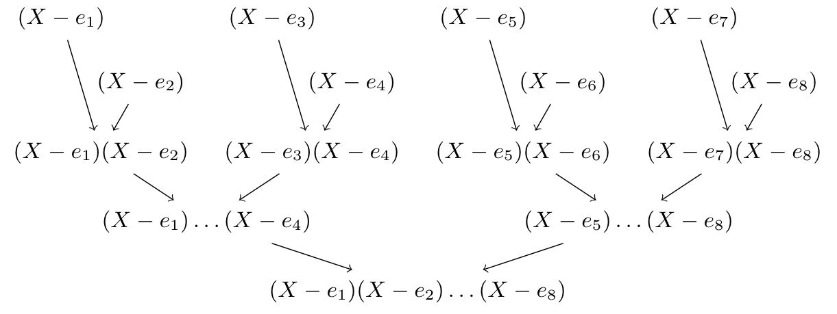
Each node in the subproduct tree multiplies the polynomials stored in its two children nodes. This way, the root polynomial will be exactly $A_I(X)$. If FFT-based multiplication is used, the time to compute a subproduct tree of size $n$ is:

\begin{align} T(n) &= 2T(n/2) + O(n\log{n})\\
&= O(n\log^2{n}) \end{align}

Observation 1: I believe computing $A_I(X)$ faster for arbitrary points $e_i$ is not possible, but I would be happy to be contradicted!

Observation 2: In practice, the algorithms for computing $R_I(X)$ and $A_I(X)$ efficiently would require FFT-based techniques for polynomial division and multiplication, and FFTs are fastest when the finite field $\Zp$ is endowed with $d$th roots of unity for sufficiently high $d$, on the order of the degrees of $R_I(X)$ and $A_I(X)$.

Verifying a batch proof

The verifier who has the commitment $c$, the evaluations $(e_i, y_i)_{i\in I}$ and a batch proof $\pi_I=g^{q_I(\tau)}$ can verify them as follows.

1. First, he interpolates the accumulator polynomial \(A_I(X)=\prod_{i\in I} (X-e_i)\) as discussed above. Then, commits to in $O(\vert I \vert)$ time: \begin{align} a &= g^{A_I(\tau)} \end{align}
2. Second, he interpolates $R_I(X)$ s.t. $R_I(e_i)=y_i,\forall i \in I$ as discussed above. Then, commits to in $O(\vert I \vert)$ time: \begin{align} r &= g^{R_I(\tau)} \end{align}
3. Third, he checks Equation \ref{eq:batch-proof-rel} holds at $X=\tau$ using two pairings: $e(c / r, g) = e(\pi_I, a)$.

Note that:

\begin{align} e(g^{\phi(\tau)} / g^{R_I(\tau)}, g) &= e(g^{q_I(\tau)}, g^{A_I(\tau)})\Leftrightarrow\\
e(g^{\phi(\tau) - R_I(\tau)}, g) &= e(g,g)^{q_I(\tau) A_I(\tau)}\Leftrightarrow\\
\phi(\tau) - R_I(\tau) &= q_I(\tau) A_I(\tau) \end{align}

Aggregation of proofs

For now, we discuss proof aggregation in a different blog post on building vector commitments (VCs) from KZG.

Applications

There are many cryptographic tools one can build using polynomial commitment schemes such as KZG.

Here’s a few we’ve blogged about in the past:

• Cryptographic accumulators
• Vector Commitments (VC) schemes with $O(\log{n})$-sized proofs or with $O(1)$-sized proofs
• Range proofs

Acknowledgements

Many thanks to Shravan Srinivasan and Philipp Jovanovic for really helping improve this post.