Towards Scalable Verifiable Secret Sharing and Distributed Key Generation

tl;dr: We “authenticate” a polynomial multipoint evaluation using Kate-Zaverucha-Goldberg (KZG) commitments. This gives a new way to precompute $n$ proofs on a degree $t$ polynomial in $\Theta(n\log{t})$ time, rather than $\Theta(nt)$.
The key trade-off is that our proofs are logarithmic-sized, rather than constant-sized. Nonetheless, we use our faster proofs to scale Verifiable Secret Sharing (VSS) protocols and distributed key generation (DKG) protocols.
We also obtain a new Vector Commitment (VC) scheme, which can be used for stateless cryptocurrencies¹.

In a previous post, I described our new techniques for scaling BLS threshold signatures to millions of signers. However, as pointed out by my friend Albert Kwon, once we have such a scalable threshold signature scheme (TSS), a new question arises:

"Can we efficiently bootstrap a $(t,n)$ threshold signature scheme when $t$ and $n$ are very large?"

The answer is: use a distributed key generation (DKG)² protocol. Unfortunately, DKGs do not scale well. Their main bottleneck is efficiently computing evaluation proofs in a polynomial commitment scheme such as KZG³. In this post, we’ll introduce new techniques for speeding this up.

As mentioned before, our full paper⁴ can be found here and will appear in IEEE S&P’20. A prototype implementation of our VSS and DKG benchmarks is available on GitHub here.

Preliminaries

Let $[n]=\{1,2,3,\dots,n\}$. Let $p$ be a sufficiently large prime that denotes the order of our groups.

In this post, beyond basic group theory for cryptographers⁵ and basic polynomial arithmetic, I will assume you are familiar with a few concepts:

• Bilinear maps⁶. Specifically, $\exists$ a bilinear map $e : \Gr_1 \times \Gr_2 \rightarrow \Gr_T$ such that:
  • $\forall u\in \Gr_1,v\in \Gr_2, a\in \Zp, b\in \Zp, e(u^a, v^b) = e(u,v)^{ab}$
  • $e(g_1,g_2)\ne 1_T$ where $g_1,g_2$ are the generators of $\Gr_1$ and $\Gr_2$ respectively and $1_T$ is the identity of $\Gr_T$
• The polynomial remainder theorem (PRT) which says that $\forall z$: $\phi(z) = \phi(X) \bmod (X-z)$,
  • Or, equivalently, $\exists q, \phi(X) = q(X)(X-z) + \phi(z)$.
    • We’ll refer to this as the PRT equation
• KZG³ polynomial commitments (see here). Specifically,
  • To commit to degree $\le \ell$ polynomials, need $\ell$-SDH public parameters $(g,g^\tau,g^{\tau^2},\dots,g^{\tau^\ell}) = (g^{\tau^i})_{i\in[0,\ell]}$,
  • Commitment to $\phi(X)=\prod_{i\in[0,d]} \phi_i X^i$ is $c=g^{\phi(\tau)}$ computed as $c=\prod_{i\in[0,\deg{\phi}]} \left(g^{\tau^i}\right)^{\phi_i}$,
  • To prove an evaluation $\phi(a) = b$, a quotient $q(X) = \frac{\phi(X) - b}{X - a}$ is computed and the evaluation proof is $g^{q(\tau)}$.
  • A verifier who has the commitment $c=g^{\phi(\tau)}$ and the proof $\pi=g^{q(\tau)}$ can verify it using a bilinear map:
    • $e(c / g^b, g) = e(\pi, g^\tau / g^a) \Leftrightarrow$
    • $e(g^{\phi(\tau)-b}, g) = e(g^{q(\tau)}, g^{\tau-a}) \Leftrightarrow$
    • $e(g,g)^{\phi(\tau)-b} = e(g,g)^{q(\tau)(\tau-a)}$.
    • This effectively checks that $q(X) = \frac{\phi(X) - b}{X-a}$ by checking this equality holds for $X=\tau$.
• The Fast Fourier Transform (FFT)⁷ applied to polynomials. Specifically,
  • Suppose $\Zp$ admits a primitive root of unity $\omega$ of order $n$ (i.e., $n \mid p-1$)
  • Let \(H=\{1, \omega, \omega^2, \omega^3, \dots, \omega^{n-1}\}\) denote the set of all $n$ $n$th roots of unity
  • Then, FFT can be used to efficiently evaluate any polynomial $\phi(X)$ at all $X\in H$ in $\Theta(n\log{n})$ time
    • i.e., compute all \(\{\phi(\omega^{i-1})\}_{i\in[n]}\)
• $(t,n)$ Verifiable Secret Sharing (VSS) via Shamir Secret Sharing. Specifically, we’ll focus on eVSS³:
  • 1 dealer with a secret $s$
  • $n$ players
  • The goal is for dealer to give each player $i$ a share $s_i$ of the secret $s$ such that any subset of $t$ shares can be used to reconstruct $s$
  • To do this, the dealer:
    • Picks a random degree $t-1$ polynomial $\phi(X)$ such that $\phi(0)=s$
    • Commits to $\phi(X)$ using KZG and broadcasts commitment $c=g^{\phi(\tau)}$ to all players
    • Gives each player $i$ its share $s_i = \phi(i)$ together with a KZG proof $\pi_i$ that the share is correct
    • Each player verifies $\pi_i$ against $c$ and its share $s_i=\phi(i)$
  • (Leaving out details about the complaint broadcasting round and the reconstruction phase of VSS.)
• $(t,n)$ Distributed Key Generation (DKG) via VSS. Specifically,
  • Just that, at a high level, a DKG protocol involves each one of the $n$ players running a VSS protocol with all the other players.

Polynomial multipoint evaluations

A key ingredient in our work, is a polynomial multipoint evaluation⁸, or a multipoint eval for short. This is just an algorithm for efficiently evaluating a degree $t$ polynomial at $n$ points in $\Theta(n\log^2{t})$ time. In contrast, the naive approach would take $\Theta(nt)$ time.

An FFT is an example of a multipoint eval, where the evaluation points are restricted to be all $n$ $n$th roots of unity. However, the multipoint eval we’ll describe below works for any set of points.

First, recall that the naive way to evaluate $\phi$ at $n$ points \(\{1,2,\dots,n\}\) is to compute:

\[\phi(i)=\sum_{j=0}^{t} \phi_j \cdot (i^j),\forall i\in[n]\]

Here, $\phi_j$ denotes the $j$th coefficient of $\phi$.

In contrast, in a multipoint eval, we will compute $\phi(i)$ by indirectly (and efficiently) computing $\phi(X) \bmod (X-i)$ which exactly equals $\phi(i)$. (Recall the polynomial remainder theorem from above.)

For example, for $n=4$, we’ll first compute a remainder polynomial: \begin{align} \color{red}{r_{1,4}(X)} &= \phi(X) \bmod (X-1)(X-2)\cdots(X-4) \end{align}

Then, we’ll “recurse”, splitting the $(X-1)(X-2)\cdots(X-4)$ vanishing polynomial into two halves, and dividing the $\color{red}{r_{1,4}}$ remainder by the two halves: \begin{align} \color{green}{r_{1,2}(X)} &= \color{red}{r_{1,4}(X)} \bmod (X-1)(X-2)\\
\color{orange}{r_{3,4}(X)} &= \color{red}{r_{1,4}(X)} \bmod (X-3)(X-4) \end{align}

A key concept in a multipoint eval is that of a vanishing polynomial over a set of points. This is just a polynomial that has roots at all those points. For example, $(X-1)(X-2)\cdots(X-4)$ is a vanishing polynomial over \(\{1,2,3,4\}\).

Finally, we’ll compute, for all \(i\in\{1,2,3,4\}\), the actual evaluations $\phi(i)$ as: \begin{align} \color{blue}{r_{1,1}(X)} &= \color{green}{r_{1,2}(X)} \bmod (X-1) = \phi(1)\\
\color{blue}{r_{2,2}(X)} &= \color{green}{r_{1,2}(X)} \bmod (X-2) = \phi(2)\\
\color{blue}{r_{3,3}(X)} &= \color{orange}{r_{3,4}(X)} \bmod (X-3) = \phi(3)\\
\color{blue}{r_{4,4}(X)} &= \color{orange}{r_{4,4}(X)} \bmod (X-4) = \phi(4) \end{align}

You might wonder how come $r_{1,1}(X)=\color{green}{r_{1,2}(X)} \bmod (X-1) = \phi(1)$? If you expand $r_{1,2}(X)$ you get $r_{1,1}(X) = \left(\left(\phi(X) \bmod (X-1)(X-2)\cdots(X-4)\right) \bmod (X-1)(X-2)\right) \bmod (X-1)$ and this is exactly equal to $\phi(X) \bmod(X-1) = \phi(1)$.

Still, a picture is worth a thousand words, so let’s depict a larger example for evaluating at \(\{1,2,3,\dots,8\}\). Importantly, we will depict divisions by the vanishing polynomials slightly differently. Specifically, rather than just focusing on the remainder and write:

\[r(X) = \phi(X) \bmod \prod_i (X-i)\]

…we focus on both the remainder and the quotient polynomial and write:

\[\phi(X) = q(X) \prod_i(X-i) + r(X)\]

Recall from your basic polynomial math that, when dividing a polynomial $a$ by another polynomial $b$, we get a quotient polynomial $q$ and a remainder polynomial $r$ of degree less than $b$ such that $a(X) = q(X) b(X) + r(X)$.

Here’s what a multipoint eval of $\phi(X)$ at \(\{1,\dots,8\}\) looks like:

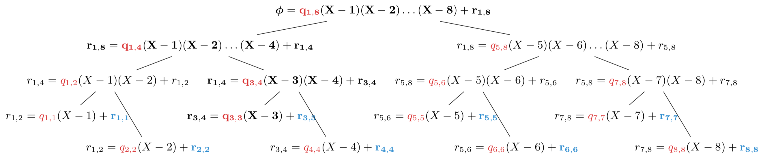
You might want to zoom in on the image above, if it’s not sufficiently clear. Each node $w$ in the multipoint eval tree stores three polynomials: a vanishing polynomial $V_w$ of the form $\prod_i (X-i)$, a quotient $q_w$ and a remainder $r_w$. If we let $u$ denote node $w$’s parent, then the multipoint evaluation operates very simply: For every node $w$, divide the parent remainder $r_u$ by $V_w$, obtaining a new remainder $r_w$ and quotient $q_w$. For the root node, the parent remainder is $\phi(X)$ itself and the vanishing polynomial is $(X-1)\cdots(X-8)$. Finally, notice that the vanishing polynomials are “split” into left and right “halves” at every node in the tree.

The end result are the remainders $r_{i,i} = \phi(X) \bmod (X-i)$ which are exactly equal to the evaluations $\phi(i)$.

It might might not be immediately obvious but, as $n$ and $t$ get large, this approach saves us a lot of work, taking only $\Theta(n\log^2{t})$ time. (In contrast, the naive approach takes $\Theta(nt)$ time.)

Hopefully, it should be clear by now that:

• A multipoint eval is used to efficiently evaluate a polynomial $\phi(X)$ at $n$ points.
• It takes $\Theta(n\log^2{t})$ time if $\phi(X)$ has degree $t$.
• The key ingredient: repeated divisions by vanishing polynomials at the evaluation points.
• These repeated divisions produce a remainder and a quotient polynomial at each node in the tree.

Authenticated Multipoint Evaluation Trees (AMTs)

In the KZG polynomial commitment scheme, computing $n$ evaluation proofs takes $\Theta(nt)$ time. Here, we will speed this up to $\Theta(n\log{t})$ time at the cost of increasing proof size from constant to logarithmic. Later on, we will use our faster proofs to help scale VSS and DKG protocols computationally, although at the cost of a small increase in communication.

The idea is very simple: we take a multipoint evaluation and “authenticate” it by committing (via KZG) to the quotient polynomials in the tree. An evaluation proof now consists of all the quotient commitments along the path to the evaluation point.

For example, in the figure above, the evaluation proof for $\phi(3)$ would be:

\[\pi_{\lvert X=3} = \left(g^{q_{1,8}(\tau)}, g^{q_{1,4}(\tau)}, g^{q_{3,4}(\tau)}, g^{q_{3,3}(\tau)}\right)\]

We call this construction an authenticated multipoint evaluation tree (AMT).

Verifying AMT proofs

What about checking a proof? Recall that, in KZG, the verifier uses the bilinear map to check that the polynomial remainder theorem (PRT) holds:

\[\exists q(X), \phi(X) = q(X)(X-3) + \phi(3)\]

Specifically, the verifier is given a commitment to $q(X)$ and checks that the property above holds at $X=\tau$ where $\tau$ is the $\ell$-SDH trapdoor.

In AMTs, the intuition remains the same, except the verifier will indirectly check the PRT holds. Specifically, for the example above, the verifier will check that, $\exists q_{1,8}(X), q_{1,4}(X), q_{3,4}(X), q_{3,3}(X)$ such that:

\begin{align} \phi(X) &=q_{1,8}(X)\cdot(X-1)\cdots(X-8) + {}\\
&+ q_{1,4}(X)\cdot(X-1)\cdots(X-4) + {}\\
&+ q_{3,4}(X)\cdot(X-3)(X-4) + {}\\
&+ q_{3,3}(X)\cdot(X-3) + {}\\
&+ \phi(3) \end{align}

We’ll refer to this as the AMT equation.

You can easily derive the AMT equation if you “expand” $\phi(X)$’s expression starting at the root and going all the way to $\phi(3)$’s leaf in the tree. \begin{align*} \phi(X) &= q_{1,8}(X)\cdot(X-1)\cdots(X-8) + r_{1,8}\\
&= q_{1,8}(X)\cdot(X-1)\cdots(X-8) + q_{1,4}(X)\cdot(X-1)\cdots(X-4) + r_{1,4}\\
&= q_{1,8}(X)\cdot(X-1)\cdots(X-8) + q_{1,4}(X)\cdot(X-1)\cdots(X-4) + q_{3,4}(X)\cdot(X-3)(X-4) + r_{3,4}\\
&= \dots %+ q_{3,3}(X)(X-3) + \phi(3) \end{align*}

Note that by factoring out $(X-3)$ in the AMT equation, we can obtain the quotient $q(X)$ that satisfies the PRT equation: \begin{align} q(X) &=q_{1,8}(X)\cdot\frac{(X-1)\cdots(X-8)}{X-3} + {}\\
&+ q_{1,4}(X)\cdot(X-1)(X-2)(X-4) + {}\\
&+ q_{3,4}(X)\cdot(X-4) + {}\\
&+ q_{3,3}(X) \end{align}

In other words, the quotient $q(X)$ from the KZG proof is just a linear combination of the quotients from the AMT proof. This is why checking the AMT equation is equivalent to checking the PRT equation.

In conclusion, to verify the AMT proof for $\phi(3)$, the verifier will use the bilinear map to ensure the AMT equation holds at $X=\tau$: \begin{align} e(g^{\phi(\tau)}, g) &= e(g^{q_{1,8}(\tau)}, g^{(\tau-1)\cdots(\tau-8)})\cdot {}\\
&\cdot e(g^{q_{1,4}(\tau)}, g^{(\tau-1)\cdots(\tau-4)})\cdot {}\\
&\cdot e(g^{q_{3,4}(\tau)}, g^{(\tau-3)(\tau-4)})\cdot {}\\
&\cdot e(g^{q_{3,3}(\tau)}, g^{\tau-3})\cdot {}\\
&\cdot e(g^{\phi(3)}, g) \end{align}

Note that for this, the verifier needs commitments to the vanishing polynomials along the path to $\phi(3)$. This means the verifer would need $O(n)$ such commitments as part of its public parameters to verify all $n$ proofs. In the paper⁴, we address this shortcoming by restricting the evaluation points to be roots of unity. This makes all vanishing polynomials be of the form $\left(X^{n/{2^i}} + c\right)$ for some constant $c$ and only requires the verifiers to have $O(\log{n})$ public parameters to reconstruct any vanishing polynomial commitment. It also has the advantage of reducing the multipoint eval time from $\Theta(n\log^2{t})$ to $\Theta(n\log{t})$.

In general, let $P$ denote the nodes along the path to an evaluation point $i$, let $w\in P$ be such a node, and $q_w, V_w$ denote the quotient and vanishing polynomials at node $w$. Then, to verify an AMT proof for $i$, the verifier will check that:

\[e(g^{\phi(\tau)}, g) = e(g^{\phi(i)}, g) \prod_{w\in P} e(g^{q_w(\tau)}, g^{V_w(\tau)})\]

By now, you should understand that:

• We can precompute $n$ logarithmic-sized evaluation proofs for a degree $t$ polynomial
  • In $\Theta(n\log^2{t})$ time, for arbitrary evaluation points
  • In $\Theta(n\log{t})$ time, if the evaluation points are roots of unity
• Verifying a proof takes logarithmic time

To be precise, the proof size and verification time are both $\Theta(\log{t})$ when $t < n$, which is the case in the VSS/DKG setting. You can see the paper⁴ for details.

Applications of AMTs

Vector commitments (VCs)

By representing a vector $v = [v_0, v_1, v_2, \dots, v_{n-1}]$ as a (univariate) polynomial $\phi(X)$ where $\phi(\omega^i) = v_i$, we can easily obtain a vector commitment scheme similar to the multivariate polynmomial-based one by Chepurnoy et al¹. Our scheme also supports updating proofs efficiently (see Chapter 9.2.2., pg. 120 in my thesis⁹ for details).

Faster VSS

Recall from the preliminaries section that the key bottleneck in eVSS is the dealer having to precompute KZG proofs for all $n$ players. This takes $\Theta(nt)$ time. By using AMTs enhanced with roots of unity, we can reduce this time to $O(n\log{t})$. This has a drastic effect on dealing time and helps scale eVSS to very large numbers of participants.

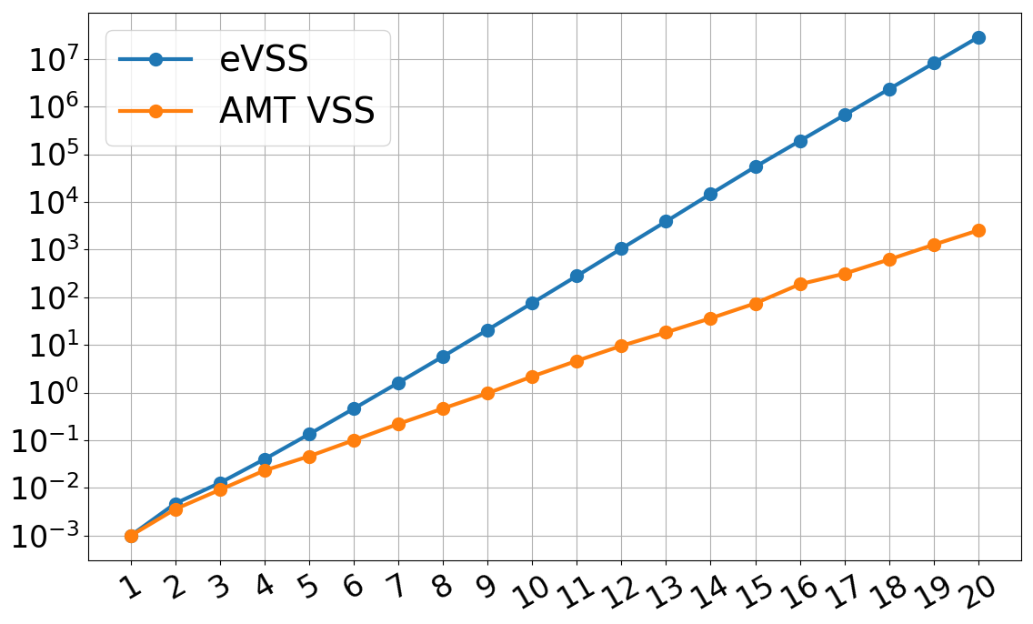
The $x$-axis is $\log_2(t)$ where $t$ is the threshold, which doubles for every tick. They $y$-axis is the dealing time in seconds. The graph shows that our AMT-based VSS outscales eVSS for large $t$ and performs better even at the scale of hundreds of players.

Faster DKG

Since in a DKG protocol, each player performs a VSS with all the other players, the results from above carry over to DKG protocols too. In fact, the DKG dealing time (per-player) doesn’t differ much from the VSS dealing time, especially as $t$ gets large. Thus, the improvement in DKG dealing times is perfectly illustrated by the graph above too.

An important thing to note here is that our AMT proofs have a homomorphic property which is necessary for using them in DKGs. Specifically, an AMT proof for $\phi(i)$ and another proof for $\psi(i)$ can be combined into a proof for $\left(\phi+\psi\right)(i)$.

Caveats

We also want to emphasize several limitations of our work:

• VSS and DKG protocols seem to inherently require a broadcast channel, which is as hard to scale as any consensus algorithm. We do not address this.
• Our results only apply to synchronous VSS and DKG protocols, which make strong assumptions about the broadcast channel.
• Our VSS and DKG protocols are not proven to be adaptively secure.
• We do not address the large communication overhead of VSS and DKG protocols deployed at large scales.

Remaining questions

Can we precompute constant-sized, rather than logarithmic-sized, KZG evaluation proofs in quasilinear time? Recently, Feist and Khovratovich¹⁰ showed this is possible if the set of evaluation points are all the $n$ $n$th roots of unity. Thus, by applying their techniques, we can further speed up computation in VSS and DKG, while maintaining the same communication efficiency. We hope to implement their techniques and see how much better than AMT VSS we can do.

Our $(t,n)$ VSS/DKG protocols require $t$-SDH public parameters. Thus, the non-trivial problem of generating $t$-SDH public parameters remains. In some sense, we make this problem worse because our scalable protocols require a large $t$. We hope to address this in future work.

References