Fast and Scalable BLS Threshold Signatures

tl;dr: We use $O(t\log^2{t})$-time algorithms to interpolate secrets “in the exponent.” This makes aggregating $(t,n)$ BLS threshold signatures much faster, both at small and large scales.

The question of scaling threshold signatures came to us at VMware Research after we finished working on SBFT¹, a scalable Byzantine Fault Tolerance (BFT) protocol that uses BLS threshold signatures².

We recently published our work³ in IEEE S&P’20. Our work also address how to scale the necessary distributed key generation (DKG) protocol needed to bootstrap a BLS threshold signature scheme. We present these results in another post.

A prototype implementation is available on GitHub here.

Preliminaries

Let $[n]=\{1,2,3,\dots,n\}$. Let $p$ be a sufficiently large prime that denotes the order of our groups.

In this post, beyond basic group theory for cryptographers⁴, I will assume you are familiar with a few concepts:

• Bilinear maps⁵. Specifically, $\exists$ a bilinear map $e : \Gr_1 \times \Gr_2 \rightarrow \Gr_T$ such that:
  • $\forall u\in \Gr_1,v\in \Gr_2, a\in \Zp, b\in \Zp, e(u^a, v^b) = e(u,v)^{ab}$
  • $e(g_1,g_2)\ne 1_T$ where $g_1,g_2$ are the generators of $\Gr_1$ and $\Gr_2$ respectively and $1_T$ is the identity of $\Gr_T$
• BLS signatures². Specifically,
  • Let $H : \{0,1\}^* \rightarrow \Gr_1$ be a collision-resistant hash-function (CRHF)
  • The secret key is $s\in_R \Zp$ and the public key is $g_2^s\in \Gr_2$
  • $\sigma = H(m)^s \in \Gr_1$ is a signature on $m$ under secret key $s$
  • To verify a signature, one checks if $e(H(m), g_2^s) = e(\sigma, g_2)$
• $(t,n)$ BLS threshold signatures⁶. Specifically,
  • Shamir secret sharing⁷ of secret key $s$
  • i.e., $s = \phi(0)$ where $\phi(X)\in \Zp[X]$ is random, degree $t-1$ polynomial
  • Signer $i\in\{1,2,\dots, n\}$ gets his secret key share $s_i = \phi(i)$ and verification key $g^{s_i}$
  • Nobody knows $s$, so cannot directly produce a signature $H(m)^s$ on $m$
  • Instead, $t$ or more signers have to co-operate to produce a signature
  • Each signer $i$ computes a signature share or sigshare $\sigma_i = H(m)^{s_i}$
  • Then, an aggregator:
    • Collects as many $\sigma_i$’s as possible
    • Verifies each $\sigma_i$ under its signer’s verification key: Is $e(H(m),g_2^{s_i}) = e(\sigma_i, g_2)$?
    • …and thus identifies $t$ valid sigshares
    • Aggregates the signature $\sigma = H(m)^s$ via “interpolation in the exponent” from the $t$ valid sigshares (see next section).

Basics of polynomial interpolation

A good source for this is Berrut and Trefethen⁸.

Let $\phi \in \Zp[X]$ be a polynomial of degree $t-1$. Suppose there are $n$ evaluations $(i, \phi(i))_{i\in [n]}$ “out there” and we have $t$ out of these $n$ evaluations. Specifically, let $(j, \phi(j))_{j \in T}$ denote this subset, where $T\subset [n]$ and $|T|=t$.

How can we recover or interpolate $\phi(X)$ from these $t$ evaluations?

We can use Lagrange’s formula, which says:

\begin{align} \phi(X) &= \sum_{j\in T} \lagr_j^T(X) \phi(j)\label{eq:lagrange-sum} \end{align}

The $\lagr_j^T(X)$’s are called Lagrange polynomials and are defined as:

\begin{align} \lagr_j^T(X) &= \prod_{\substack{k\in T\\k\ne j}} \frac{X - k}{j - k}\label{eq:lagrange-poly} \end{align}

The key property of these polynomials is that $\forall j\in T, \lagr_j^T(j) = 1$ and $\forall i\in T, i\ne j,\lagr_j^T(i) = 0$.

We are artificially restricting ourselves to evaluations of $\phi$ at points $\{1,2,\dots,n\}$ since this is the setting that arises in BLS threshold signatures. However, these protocols work for any set of points $(x_i, \phi(x_i))_{i\in [n]}$. For example, as we’ll see later, it can be useful to replace the signer IDs $\{1,2,\dots,n\}$ with roots of unity $\{\omega^0, \omega^1, \dots, \omega^{n-1}\}$.

Faster BLS threshold signatures

As explained before, aggregating a $(t,n)$ threshold signature such as BLS, requires interpolating the secret key $s$ “in the exponent.” This is typically done naively in $\Theta(t^2)$ time.

In our paper³, we adapt well-known, fast polynomial interpolation algorithms⁹ to do this in $O(t\log^2{t})$ time. This not only scales BLS threshold signature aggregation to millions of signers, but also speeds up aggregation at smaller scales of hundreds of signers.

First, I’ll describe the naive, quadratic-time algorithm for aggregation. Then, I’ll introduce the quasilinear-time algorithm, adapted for the “in the exponent” setting.

Quadratic-time BLS threshold signature aggregation

Having identified $t$ valid signature shares $\sigma_j = H(m)^{s_j}, j\in T$, the aggregator will recover $s=\phi(0)$ but do so “in the exponent”, by recovering $H(m)^{\phi(0)}=H(m)^s$.

For this, the aggregator computes all the $\lagr_j^T(0)$’s by computing Equation $\ref{eq:lagrange-poly}$ at $X=0$:

\[\lagr_j^T(0) = \prod_{\substack{k\in T\\\\k\ne j}} \frac{0 - k}{j - k} = \prod_{\substack{k\in T\\\\k\ne j}} \frac{k}{k - j}\]

Computing a single $\lagr_j^T(0)$ can be done in $\Theta(t)$ time by simply carrying out the operations above in the field $\Zp$. However, we need to compute all of them: $\lagr_j^T(0), \forall j \in T$, which takes $\Theta(t^2)$ time. We will describe how to reduce this time in the next subsection.

The final step consists of several exponentiations in $\Gr_1$, which actually computes the secret key $s$ in the exponent, as per Equation \ref{eq:lagrange-sum} at $X=0$:

\begin{align} \prod_{j\in T} \sigma_j^{\lagr_j^T(0)} &= \prod_{j\in T} \left(H(m)^{s_j}\right)^{\lagr_j^T(0)}\\
&= \prod_{j\in T} H(m)^{\lagr_j^T(0) s_j}\\
&= H(m)^{\sum_{j\in T}{\lagr_j^T(0) s_j}}\\
&= H(m)^{\sum_{j\in T}{\lagr_j^T(0) \phi(j)}}\\
&= H(m)^{\phi(0)} = H(m)^s = \sigma \end{align}

This last step takes $\Theta(t)$ time and is sped up in practice using multi-exponentiation techniques.

This naive algorithm works quite well, especially at small scales, but the performance deteriorates fast, as computing the $\lagr_j^T(0)$’s becomes very expensive. The figure below depicts this trend.

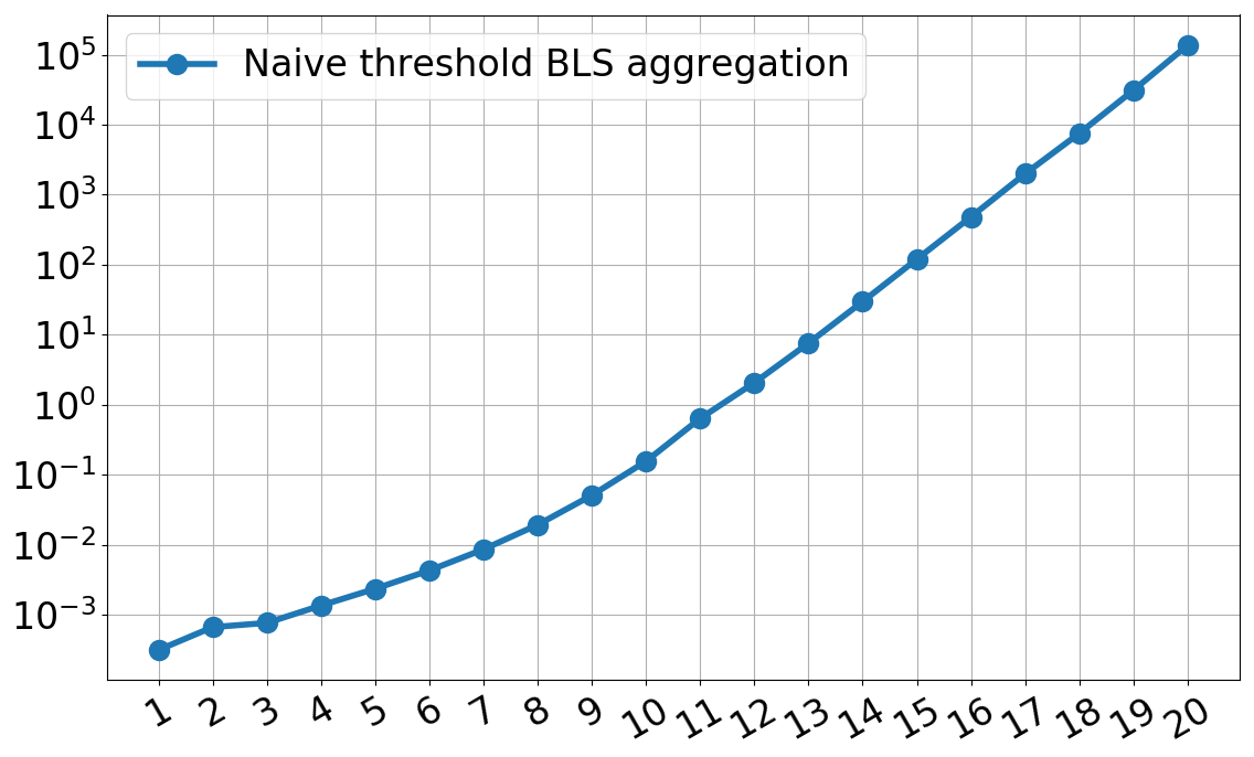
The $x$-axis is $\log_2(t)$ where $t$ is the threshold, which doubles for every tick. The $y$-axis is the time to aggregate a $(t, 2t-1)$ BLS threshold signature in seconds. This consists of (1) the time to compute the Lagrange coefficients and (2) the time to compute the multi-exponentiation. As you can see, for $t=2^{11}=2048$, the time to aggregate is less than 1 second.

The BLS threshold signature aggregation code was implemented using libff and libfqfft and is available on GitHub here. We used various optimizations using roots-of-unity to speed up this naive implementation.

Our quasilinear-time BLS threshold signature aggregation

This is going to get a bit mathematical, so hold on tight. Everything explained here is just a slight modification of the fast polynomial interpolation techniques explained in “Modern Computer Algebra”⁹.

We’ll refer to $\lagr_j^T(0)$ as a Lagrange coefficient: this is just the Lagrange polynomial from Equation \ref{eq:lagrange-poly} evaluated at $X=0$. Recall that the aggregator must compute all $t=|T|$ Lagrange coefficients.

Step 1: Numerators and denominators of Lagrange coefficients

Notice that each Lagrange coefficient can be rewritten as a numerator divided by a denominator. All $t$ numerators can be computed very fast in $\Theta(t)$ time, but the denominators will be a bit more challenging.

First, we define a vanishing polynomial $V_T(X)$ that has roots at all $X\in T$: \begin{align} V_T(X) = \prod_{j\in T} (X - j) \end{align}

Similarly, let $V_{T\setminus\{j\}}(X)$ have roots at all $X\in T\setminus\{j\}$: \begin{align} V_{T\setminus\{j\}}(X) =\prod_{\substack{k\in T\\k\ne j}} (X - k)=V_T(X)/(X - j) \end{align}

Second, we rewrite the Lagrange polynomials using these vanishing polynomials. \begin{align} \lagr_j^T(X) &= \prod_{\substack{k\in T\\k\ne j}} \frac{X - k}{j - k}\\
&= \frac{\prod_{\substack{k\in T\\k\ne j}}(X - k)}{\prod_{\substack{k\in T\\k\ne j}}(j - k)}\\
&= \frac{V_{T\setminus\{j\}}(X)}{V_{T\setminus\{j\}}(j)} \end{align}

As a result, we can rewrite the Lagrange coefficients as: \begin{align} \lagr_j^T(0) &= \frac{V_{T\setminus\{j\}}(0)}{V_{T\setminus\{j\}}(j)} \end{align}

Finally, we note that computing all numerators $V_{T\setminus\{j\}}(0)=V_T(0)/(0-j)$ can be done in $\Theta(t)$ time by:

1. Computing $V_T(0)$ in $\Theta(t)$ time

2. Dividing it by $-j$ for all $j\in T$, also in $\Theta(t)$ time

Step 2: Computing all denominators $\Leftrightarrow$ evaluate some polynomial at $t$ points

(It is a bit more difficult to) notice that the denominator $V_{T\setminus\{j\}}(j)$ equals exactly $V_T’(j)$, where $V_T’$ is the derivative of $V_T$. This means that we can compute all denominators by evaluating $V_T’$ at all $j\in T$. We will explain later how we can do this evaluation very efficiently.

First, let us see what $V_T’(X)$ looks like. Here, it’s helpful to take an example. Say $T = \{1,3,9\}$ (i.e., the aggregator identified 3 valid sigshares from players 1, 3 and 9), which means $V_T(X)=(X-1)(X-3)(x-9)$.

If we apply the product rule of differentiation, we get: \begin{align} V_T’(x) &= \big[(x-1)(x-3)\big]'(x-9) + \big[(x-1)(x-3)\big](x-9)’\\
&= \big[(x-1)’(x-3) + (x-1)(x-3)’\big](x-9) + (x-1)(x-3)\\
&= \big[(x-3)+(x-1)\big](x-9) + (x-1)(x-3)\\
&= (x-3)(x-9) + (x-1)(x-9) + (x-1)(x-3)\\
&= V_{T\setminus\{1\}}(x) + V_{T\setminus\{3\}}(x) + V_{T\setminus\{9\}}(x) \end{align}

In general, for any set $T$ of signers, it is the case that: \begin{align} V_T’(X) = \sum_{k \in T} V_{T\setminus\{k\}}(X) \end{align}

We leave proving this as an exercise. The example above should give you enough intuition for why this holds.

Second, notice that $V_T’(j) = V_{T\setminus\{j\}}(j)$ does appear to hold for this example where $T=\{1,3,9\}$: \begin{align} V_T’(1) &= (1-3)(1-9) + 0 + 0 = V_{T\setminus\{1\}}(1)\\
V_T’(3) &= 0 + (3-1)(3-9) + 0 = V_{T\setminus\{3\}}(1)\\
V_T’(9) &= 0 + 0 + (9-1)(9-3) + 0 = V_{T\setminus\{9\}}(1) \end{align}

We can easily prove this holds for any set $T$ of signers: \begin{align} V_T’(j) &= \sum_{k \in T} V_{T\setminus\{k\}}(j)\\
&= V_{T\setminus\{j\}}(j) + \sum_{k \in T\setminus\{j\}} V_{T\setminus\{k\}}(j)\label{eq:vtprimeofj}\\
&= V_{T\setminus\{j\}}(j) + \sum_{k \in T\setminus\{j\}} 0\label{eq:vtprimeofj-zero}\\\ &= V_{T\setminus\{j\}}(j) \end{align}

In other words, this means the denominator of the $j$th Lagrange coefficient $\lagr_j^T(0)$ exactly equals $V_T’(j)$, as we promised in the beginning.

If you missed the transition from Equation \ref{eq:vtprimeofj} to Equation \ref{eq:vtprimeofj-zero} recall that $V_{T\setminus\{k\}}(X)$ is zero for all $X$ in $T$ except for $k$. Thus, since $j \in T$ and $j\ne k$, we have $V_{T\setminus\{k\}}(j) = 0$.

Step 3: Evaluating $V_T’(X)$ fast at all $X\in T$

The road so far (to fast BLS threshold signature aggregation):

• Compute all numerators in $O(t)$ time
• Compute the vanishing polynomial $V_T(X)$ in $O(t\log^2{t})$ time. How?
  • Build a tree!
  • Each leaf stores a monomial $(X-j)$, for all $j\in T$
  • The parent of two nodes stores the product of their children’s polynomials
  • As a result, the root will store $V_T(X)$
  • (See an example figure below for $T=\{2,4,5,8,9,13,16,20\}$.)
• Compute its derivative $V_T’(X)$ in $O(t)$ time. How?
  • Rewrite $V_T(X)$ in coefficient form as $V_T(X) = \sum_{i=0}^{|T|} c_i X^i$
  • Then, $V_T’(X) = \sum_{i=1}^{|T|} i \cdot c_i \cdot X^{i-1}$
• Evaluate $V_T’(X)$ at all points in $T$. Let’s see how!

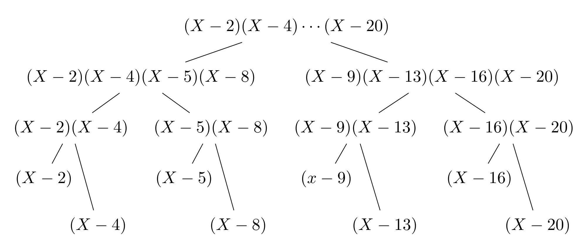
Here we are computing $V_T(X)$ when $T=\{2,4,5,8,9,13,16,20\}$. At each node in the tree, the two children’s polynomials are being multiplied. Multiplication can be done fast in $O(d\log{d})$ time using the Fast Fourier Transform (FFT)¹⁰, where $d$ is the degree of the children polynomials.

Evaluate $V_T’(X)$ using a polynomial multipoint evaluation

We want to evaluate $V_T’(X)$ of degree $t-1$ at $t$ points: i.e., at all $j\in T$. If we do this naively, one evaluation takes $\Theta(t)$ time and thus all evaluations take $\Theta(t^2)$ time. Fortunately, a $\Theta(t\log^2{t})$ algorithm exists and is called a polynomial multipoint evaluation⁹, or a multipoint eval for short.

To understand how a multipoint eval works, first you must understand two things:

1. The polynomial remainder theorem, which says $\forall$ polynomials $\phi$ and $\forall j$, $\phi(j) = \phi(X) \bmod (X-j)$, where $\bmod$ is the remainder of the division $\phi(X) / (X-j)$.
   • We’ll refer to these operations as “modular reductions.”
2. Recursion!

A multipoint eval computes $\phi(j)$ by recursively computing $\phi(X) \bmod (X-j)$ in an efficient manner. Since a picture is worth a thousands words, please take a look at the figure below, which depicts a multipoint eval of $\phi$ at $T=\{1,2,\dots,8\}$.

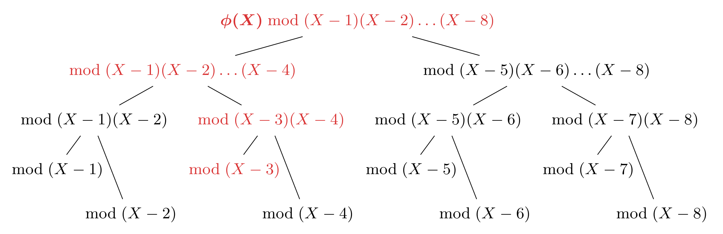
Each node $w$ in the multipoint eval tree stores two polynomials: a vanishing polynomial $V_w$ and a remainder $r_w$. If we let $u$ denote node $w$’s parent, then the multipoint evaluation operates as follows: For every node $w$, compute $r_w = r_u \bmod V_w$. (In the tree, this is depicted more simply using a “$\text{mod}\ V_w$” at each node $w$.) To start the recursive computation, the root node $\varepsilon$ has $r_\varepsilon=\phi(X)\bmod (X-1)(X-2)\cdots(X-8)$. The other important rule is for every node $w$, the children of node $w$ will store the “left” and “right” halves of $V_w$. This helps split the problem into two halves and halves the degree of the remainders at each level.

Each path in the tree corresponds to a sequence of modular reductions applied to $\phi$, ultimately leading to an evaluation $\phi(j)$. For example, the red path to $\bmod (X-3)$ gives the evaluation $\phi(3)$ and corresponds to the following sequence of modular reductions:

\[\big(\left[\left(\phi(X) \bmod (X-1)\dots(X-8)\right)\bmod(X-1)\dots(X-4)\right]\bmod(X-3)(X-4)\big)\bmod(X-3)\]

My explanation here is in many ways inadequate. Although the figure should be of some help, you should see “Modern Computer Algebra”, Chapter 10⁹ and our paper³ for more background on polynomial multipoint evaluations.

By reasoning about the degrees of the polynomials involved in the tree, one can show that at most $O(t\log{t})$ work is being done at each level in the multipoint eval tree. Since there are roughly $\log{t}$ levels, this means the multipoint eval only takes $O(t\log^2{t})$ time.

In practice, a multipoint eval requires implementing fast polynomial division using FFT. Next, we explain how to avoid this and get a considerable speed-up.

Evaluate $V_T’(X)$ using the Fast Fourier Transform (FFT)

If we pick the signer IDs to be roots of unity rather than $\{1,2,\dots,n\}$, we can evaluate $V_T’(X)$ fast in $\Theta(n\log{n})$ time with a single Fast Fourier Transform (FFT). For example, let $\omega$ be a primitive $N$th root of unity (where $N$ is the smallest power of 2 that is $\ge n$). Then, signer $i$ could have ID $\omega^{i-1}$ rather than $i$. This would slightly change the definitions of the Lagrange polynomials and the vanishing polynomials too: they would be of the form $\prod_{j\in T}(X-\omega_N^{j-1})$ rather than $\prod_{j\in T}(X - j)$.

This is actually the route we take in our paper³, since a single FFT will be much faster than a polynomial multipoint evaluation which requires multiple polynomial divisions, which in turn require multiple FFTs. You can see the performance boost and scalability gained in the figure below.

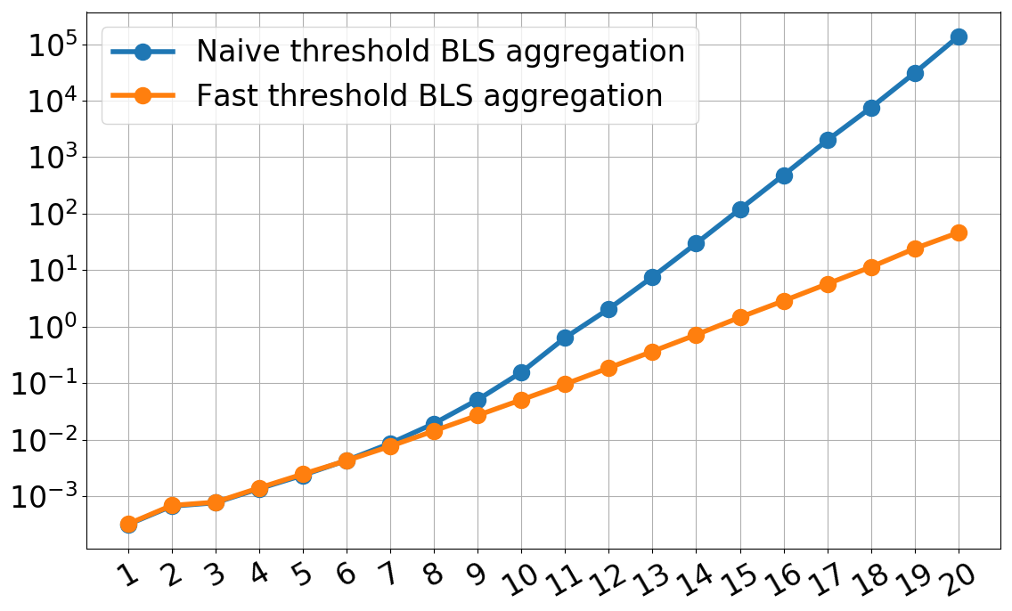
The $x$-axis is $\log_2(t)$ where $t$ is the threshold, which doubles for every tick. The $y$-axis is the time to aggregate, using the quasilinear-time Lagrange algorithm, a $(t, 2t-1)$ BLS threshold signature in seconds. As you can see, for $t=2^{11}=2048$, the time to aggregate decreases from 1 second to 0.1 seconds. We also scale better: in 1 second we can aggregate a signature with $t=2^{14}\approx 16,000$. Furthermore, we get a performance boost even at scales as small as $t=128$.

Again, the code is available on GitHub here.

Ending notes

We showed how existing algorithms for polynomial interpolation can (and should) be used to speed up and scale BLS threshold signatures. In fact, these techniques can be applied to any threshold cryptosystem whose secret lies in a prime-order finite field with support for roots of unity.

References